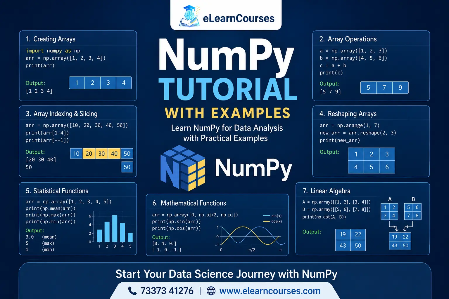
NumPy Tutorial with Examples
If you’ve ever tried looping through a Python list to add two sets of numbers together and noticed it felt slower than it should, NumPy is the reason that problem stops existing. This NumPy tutorial with examples covers everything from creating your first array to matrix operations, with runnable code at every step, so you can follow along in your own Python environment as you go.
NumPy (Numerical Python) is the foundation almost every data science and machine learning library in Python is built on top of. Pandas, scikit-learn, TensorFlow, and PyTorch all rely on NumPy arrays or something modeled closely on them, which makes it one of the highest-leverage libraries to actually understand rather than just use through a wrapper.
Why NumPy Instead of Regular Python Lists
Python lists are flexible, but that flexibility comes at a cost. Each element in a list is a separate Python object, stored with its own memory overhead, and operations on lists usually require looping through elements one at a time in Python itself, which is slow compared to compiled code.
NumPy arrays store data in a single contiguous block of memory, all of one fixed type, and operations run using precompiled C code under the hood instead of a Python loop. The practical result: NumPy operations on large arrays run many times faster than the equivalent pure Python code, and the syntax for expressing those operations is often shorter too.
import time
import numpy as np

size = 1_000_000
python_list = list(range(size))
numpy_array = np.arange(size)

start = time.time()
python_result = [x * 2 for x in python_list]
print("Python list time:", time.time() - start)

start = time.time()
numpy_result = numpy_array * 2
print("NumPy array time:", time.time() - start)
Run this yourself and the NumPy version will typically finish several times faster, sometimes more, depending on your machine. That speed difference becomes significant once you’re working with real datasets rather than toy examples.
Installing NumPy
If you don’t already have NumPy installed:
pip install numpyThen import it in your scripts using the standard convention:
import numpy as npNearly every NumPy tutorial and every codebase that uses NumPy imports it as np, so it’s worth adopting that convention from the start rather than inventing your own.
Creating NumPy Arrays
There are several ways to create arrays, depending on what you’re starting with.
import numpy as np

# From a Python list
arr = np.array([1, 2, 3, 4, 5])
print(arr)

# 2D array from a list of lists
matrix = np.array([[1, 2, 3], [4, 5, 6]])
print(matrix)

# Array of zeros
zeros = np.zeros((3, 4))

# Array of ones
ones = np.ones((2, 2))

# Array with a range of values
ranged = np.arange(0, 10, 2)  # start, stop, step
print(ranged)  # [0 2 4 6 8]

# Evenly spaced values between two numbers
spaced = np.linspace(0, 1, 5)  # 5 values between 0 and 1
print(spaced)  # [0.   0.25 0.5  0.75 1.  ]

# Random array
random_arr = np.random.rand(3, 3)
np.arange is similar to Python’s built-in range, but returns an actual array. np.linspace is useful when you need a specific number of evenly spaced points rather than a specific step size, which comes up constantly in plotting and simulations.
Array Attributes: Shape, Size, and Data Type
Every NumPy array carries metadata about its structure, which is useful for debugging and for writing code that adapts to different input sizes.
arr = np.array([[1, 2, 3], [4, 5, 6]])

print(arr.shape)   # (2, 3) - 2 rows, 3 columns
print(arr.ndim)    # 2 - number of dimensions
print(arr.size)    # 6 - total number of elements
print(arr.dtype)   # int64 (or int32, depending on platform)
shape is the attribute you’ll check most often, especially when debugging a mismatch between two arrays you’re trying to combine. dtype matters because NumPy arrays are strictly typed. Mixing integers and floats in the same array causes everything to be upcast to floats, which is worth knowing before it causes a confusing bug in a calculation you expected to stay in integers.
Choosing the Right Data Type
NumPy supports several numeric types, and picking the right one affects both memory usage and calculation accuracy.
int_arr = np.array([1, 2, 3], dtype=np.int32)
float_arr = np.array([1.5, 2.5], dtype=np.float64)
small_int = np.array([1, 2, 3], dtype=np.int8)  # -128 to 127 only

print(int_arr.nbytes)    # 12 (3 elements x 4 bytes each)
print(small_int.nbytes)  # 3 (3 elements x 1 byte each)
The default types, int64 and float64 on most systems, work fine for everyday scripts. But once you’re working with large arrays, for example millions of pixel values in image data, choosing a smaller type like int8 or float32 can meaningfully cut down memory usage. The tradeoff is range and precision: int8 can only hold values from -128 to 127, and using it for data outside that range causes silent overflow rather than an error, which is a genuinely easy mistake to make without noticing.
You can convert between types explicitly using .astype():
arr = np.array([1.9, 2.1, 3.7])
int_version = arr.astype(np.int32)
print(int_version)  # [1 2 3] - truncated, not rounded
Note that converting float to int truncates the decimal rather than rounding, so 2.9 becomes 2, not 3. Use np.round() before converting if you actually want rounding behavior.
Indexing and Slicing Arrays
NumPy indexing extends Python’s normal list indexing to handle multiple dimensions.
arr = np.array([10, 20, 30, 40, 50])
print(arr[0])       # 10
print(arr[-1])      # 50
print(arr[1:4])     # [20 30 40]

matrix = np.array([[1, 2, 3], [4, 5, 6], [7, 8, 9]])
print(matrix[0, 2])     # 3 (row 0, column 2)
print(matrix[1, :])     # [4 5 6] - entire second row
print(matrix[:, 0])     # [1 4 7] - entire first column
print(matrix[0:2, 1:3]) # [[2 3] [5 6]] - submatrix
The comma-separated indexing (matrix[1, :]) is the part that trips up people coming from plain Python lists, since a nested Python list would need matrix[1][:] instead. NumPy’s combined syntax is more compact once it’s familiar.
Boolean Indexing
Boolean indexing is one of the most useful features in NumPy, letting you filter an array based on a condition without writing an explicit loop.
arr = np.array([1, 2, 3, 4, 5, 6, 7, 8])
mask = arr > 4
print(mask)          # [False False False False True True True True]
print(arr[mask])     # [5 6 7 8]

# Combine directly
print(arr[arr % 2 == 0])  # [2 4 6 8]
Fancy Indexing
You can also index using a list or array of specific positions:
arr = np.array([10, 20, 30, 40, 50])
indices = [0, 2, 4]
print(arr[indices])  # [10 30 50]
Reshaping Arrays
Changing an array’s shape without changing its data is a common step before feeding data into a machine learning model or a plotting function.
arr = np.arange(12)
print(arr)  # [0 1 2 3 4 5 6 7 8 9 10 11]

reshaped = arr.reshape(3, 4)
print(reshaped)

flattened = reshaped.flatten()
print(flattened)  # back to a 1D array

transposed = reshaped.T
print(transposed)  # rows and columns swapped
reshape requires the total number of elements to stay the same, so a 12-element array can become 3×4 or 4×3 or 2×6, but not 3×5. Using -1 as one of the dimensions tells NumPy to calculate that dimension automatically:
auto_reshaped = arr.reshape(3, -1)  # NumPy figures out the second dimension
print(auto_reshaped.shape)  # (3, 4)
Array Operations and Broadcasting
Arithmetic on NumPy arrays works element-by-element by default, which is different from how it works on Python lists.
a = np.array([1, 2, 3])
b = np.array([10, 20, 30])

print(a + b)   # [11 22 33]
print(a * b)   # [10 40 90]
print(a ** 2)  # [1 4 9]
Compare that to Python lists, where a + b would concatenate the lists instead of adding elements, and a * b would raise an error entirely. This element-wise behavior is one of the main reasons NumPy syntax feels more natural for numerical work.
Broadcasting Explained
Broadcasting is NumPy’s set of rules for performing operations between arrays of different shapes, without you needing to manually resize anything.
matrix = np.array([[1, 2, 3], [4, 5, 6]])
vector = np.array([10, 20, 30])

result = matrix + vector
print(result)
# [[11 22 33]
#  [14 25 36]]
Here, the 1D vector gets applied to each row of the 2D matrix automatically. NumPy compares shapes dimension by dimension, starting from the last one, and two dimensions are compatible if they’re equal or if one of them is 1. A shape of (2, 3) and a shape of (3,) are compatible because NumPy treats the vector as if it had shape (1, 3) and stretches it across both rows.
Broadcasting fails, and raises an error, when shapes genuinely don’t align:
mismatched = np.array([1, 2])  # shape (2,)
try:
    matrix + mismatched  # matrix is (2, 3), this won't broadcast
except ValueError as e:
    print("Broadcasting error:", e)
Understanding broadcasting rules well enough to predict when they’ll work saves a lot of time debugging shape errors later, especially once arrays have three or more dimensions.
Universal Functions (ufuncs)
Universal functions, usually called ufuncs, are NumPy operations that apply element-wise across an entire array, and most of the math module’s equivalents have a NumPy version built for arrays instead of single numbers.
arr = np.array([1, 4, 9, 16, 25])

print(np.sqrt(arr))   # [1. 2. 3. 4. 5.]
print(np.exp(arr))    # e raised to each element
print(np.log(arr))    # natural log of each element
print(np.abs(np.array([-3, -1, 2, -5])))  # [3 1 2 5]
These run considerably faster than applying Python’s built-in math module functions in a loop, since ufuncs are implemented in compiled code and operate on the whole array in one pass rather than one value at a time.
Conditional Logic With np.where
np.where applies a condition across an array and returns different values depending on whether each element passes it, which is a common alternative to writing a loop with an if statement inside it.
arr = np.array([1, -2, 3, -4, 5, -6])

result = np.where(arr > 0, arr, 0)
print(result)  # [1 0 3 0 5 0] - negative values replaced with 0

# Get the indices where a condition is true
positive_indices = np.where(arr > 0)
print(positive_indices)  # (array([0, 2, 4]),)
This pattern, replacing negative values, capping values at a threshold, or flagging outliers, comes up constantly in real data cleaning work, and np.where handles it in a single vectorized line instead of an explicit loop.
Mathematical and Statistical Functions
NumPy includes a large set of built-in functions for common calculations, all implemented efficiently across entire arrays at once.
arr = np.array([4, 8, 15, 16, 23, 42])

print(np.sum(arr))       # 108
print(np.mean(arr))      # 18.0
print(np.median(arr))    # 15.5
print(np.std(arr))       # standard deviation
print(np.min(arr), np.max(arr))  # 4 42
print(np.argmin(arr), np.argmax(arr))  # index of min (0) and max (5)
For 2D arrays, most of these functions accept an axis argument to control whether the calculation runs across rows, columns, or the whole array:
matrix = np.array([[1, 2, 3], [4, 5, 6]])

print(np.sum(matrix))          # 21 - sum of everything
print(np.sum(matrix, axis=0))  # [5 7 9] - sum down each column
print(np.sum(matrix, axis=1))  # [6 15] - sum across each row
Getting axis=0 and axis=1 backwards is a common early mistake. axis=0 moves down the rows (producing one result per column), and axis=1 moves across the columns (producing one result per row).
Combining and Splitting Arrays
a = np.array([1, 2, 3])
b = np.array([4, 5, 6])

print(np.concatenate([a, b]))  # [1 2 3 4 5 6]

matrix1 = np.array([[1, 2], [3, 4]])
matrix2 = np.array([[5, 6], [7, 8]])

print(np.vstack([matrix1, matrix2]))  # stacked vertically
print(np.hstack([matrix1, matrix2]))  # stacked side by side

arr = np.arange(9)
split_arrays = np.split(arr, 3)
print(split_arrays)  # three arrays of length 3
vstack and hstack are shortcuts for the most common concatenation directions, and both are used constantly when assembling datasets from smaller pieces.
Sorting Arrays
arr = np.array([5, 2, 8, 1, 9, 3])
print(np.sort(arr))            # [1 2 3 5 8 9]
print(np.argsort(arr))         # indices that would sort the array

matrix = np.array([[3, 1], [2, 4]])
print(np.sort(matrix, axis=0))  # sort each column independently
argsort is particularly useful when you need to sort one array based on the order of another, for example sorting a list of names based on associated scores.
Linear Algebra with NumPy
NumPy’s linalg module covers most linear algebra operations you’ll need for machine learning and scientific computing.
A = np.array([[1, 2], [3, 4]])
B = np.array([[5, 6], [7, 8]])

# Matrix multiplication
print(np.dot(A, B))
print(A @ B)  # equivalent, more common in modern code

# Transpose
print(A.T)

# Determinant
print(np.linalg.det(A))

# Inverse
print(np.linalg.inv(A))

# Solving a system of linear equations: Ax = b
b = np.array([1, 2])
x = np.linalg.solve(A, b)
print(x)
The @ operator for matrix multiplication was introduced specifically to make linear algebra code more readable, and it’s now the more common way to write matrix multiplication in modern NumPy and PyTorch code, rather than calling np.dot explicitly.
Working With Random Numbers
NumPy’s random module is used constantly for simulations, initializing machine learning model weights, and generating test data.
np.random.seed(42)  # makes results reproducible

print(np.random.rand(3))        # 3 random floats between 0 and 1
print(np.random.randint(1, 100, size=5))  # 5 random integers from 1-99
print(np.random.normal(0, 1, size=5))     # 5 values from a normal distribution
Setting a seed with np.random.seed() is worth doing in any tutorial, test, or experiment where you need the same “random” results every time you run the code, which matters for debugging and for anyone trying to reproduce your results later.
Saving and Loading NumPy Arrays
Once you’ve built or processed an array, you’ll often need to save it for later rather than regenerating it every time a script runs.
arr = np.array([1, 2, 3, 4, 5])

# Save in NumPy's own binary format (fast, compact, NumPy-specific)
np.save('my_array.npy', arr)
loaded = np.load('my_array.npy')
print(loaded)

# Save as plain text (readable, portable, larger file size)
np.savetxt('my_array.txt', arr)
loaded_txt = np.loadtxt('my_array.txt')
print(loaded_txt)

# Save multiple arrays together
np.savez('multiple_arrays.npz', first=arr, second=arr * 2)
data = np.load('multiple_arrays.npz')
print(data['first'], data['second'])
.npy and .npz formats are the better choice when you’re staying entirely within NumPy or Python, since they preserve data types exactly and load faster. savetxt is worth using when you need the file to be human-readable or opened in something other than Python, though it’s slower and produces larger files for the same data.
Handling Missing Values
Real-world data almost always has gaps, and NumPy represents a missing numeric value using np.nan (Not a Number).
arr = np.array([1, 2, np.nan, 4, np.nan, 6])

print(np.isnan(arr))         # [False False True False True False]
print(np.sum(np.isnan(arr))) # 2 - count of missing values

# Regular functions propagate NaN through the whole result
print(np.mean(arr))    # nan

# The nan-aware versions ignore missing values instead
print(np.nanmean(arr)) # 3.25
print(np.nansum(arr))  # 13.0
This trips up a lot of people the first time: calling np.mean() on an array containing even a single nan returns nan for the entire calculation, not just for that one value. Whenever a dataset might contain missing values, reaching for the nan-prefixed version of a function (nanmean, nansum, nanstd, and so on) avoids that silent failure.
Set Operations on Arrays
NumPy includes set-style operations that work directly on arrays, which is useful for comparing groups of values without converting to Python sets first.
a = np.array([1, 2, 3, 4, 5])
b = np.array([3, 4, 5, 6, 7])

print(np.unique(a))            # removes duplicates, returns sorted values
print(np.intersect1d(a, b))    # [3 4 5] - values in both
print(np.union1d(a, b))        # [1 2 3 4 5 6 7] - all unique values combined
print(np.setdiff1d(a, b))      # [1 2] - in a but not in b
print(np.in1d(a, b))           # [False False True True True] - membership check
np.unique is particularly common for a quick check of distinct categories or labels in a dataset before deciding how to encode or group them.
Common NumPy Mistakes to Avoid
Confusing reshape requirements. The total element count must match, and forgetting this produces a ValueError that’s easy to trace once you know to check it.
Modifying a view without meaning to. Slicing a NumPy array often returns a view, not a copy, so changing the sliced version can silently change the original array too. Use .copy() explicitly when you need an independent version:
arr = np.array([1, 2, 3, 4, 5])
view = arr[1:3]
view[0] = 99
print(arr)  # [1 99 3 4 5] - the original changed too

safe_copy = arr[1:3].copy()
safe_copy[0] = 0
print(arr)  # unaffected this time
Mixing data types unintentionally. Adding a float to an integer array upcasts the whole array to floats, which can quietly break code that assumed integer indices or counts further downstream.
Looping instead of vectorizing. Writing a Python for loop over a NumPy array to do something already available as a built-in operation defeats most of the performance benefit NumPy exists to provide. If you find yourself writing a loop over array elements, it’s worth checking whether a vectorized NumPy function already does the same thing.
A Quick Look at NumPy for Image Data
Images are one of the more intuitive places to see NumPy arrays in action, since a grayscale image is really just a 2D array of brightness values, and a color image is a 3D array with an extra dimension for red, green, and blue channels.
import numpy as np

# A tiny 4x4 grayscale "image", values from 0 (black) to 255 (white)
image = np.array([
    [0, 50, 100, 150],
    [50, 100, 150, 200],
    [100, 150, 200, 250],
    [150, 200, 250, 255]
])

# Invert the image (like a photo negative)
inverted = 255 - image
print(inverted)

# Brighten the image, capping at 255 so values don't overflow
brightened = np.clip(image + 60, 0, 255)
print(brightened)
np.clip restricts every value in an array to a given range, which is exactly what’s needed here to stop brightened pixel values from wrapping around past 255. This same array-based thinking scales up directly to real photos loaded through libraries like Pillow or OpenCV, both of which represent images as NumPy arrays under the hood, so everything covered in this NumPy tutorial’s examples applies just as well to actual image processing work.
Practice Project
A solid way to put this NumPy tutorial’s examples into practice: load a small CSV of numeric data (temperatures, sales figures, or test scores work fine) into a NumPy array, then calculate the mean, median, and standard deviation, filter out outliers using boolean indexing, normalize the values to a 0-1 range using broadcasting, and finally sort the results. That single exercise touches array creation, statistical functions, boolean indexing, and broadcasting, which covers most of what you’ll actually use day to day.
Frequently Asked Questions
Is NumPy the same as pandas? No. NumPy provides the core array data structure and mathematical operations. Pandas is built on top of NumPy and adds labeled rows and columns, missing-data handling, and tools better suited to tabular data specifically. Most real projects use both together.
Do I need to learn NumPy before machine learning? Yes, in practice. Libraries like scikit-learn, TensorFlow, and PyTorch all expect data in array formats closely related to NumPy arrays, and understanding shapes, broadcasting, and indexing makes debugging model code far more manageable.
Why are NumPy arrays faster than Python lists? NumPy arrays store data in a single contiguous block of memory, all of the same type, and operations run using precompiled, optimized code rather than a Python-level loop. That combination is what produces the speed difference shown earlier in this tutorial.
What does “vectorization” mean in NumPy? It means expressing an operation across an entire array at once, using NumPy’s built-in functions, instead of writing an explicit loop over individual elements. Vectorized code is both faster and typically shorter than the equivalent loop-based version.
Can NumPy handle more than two dimensions? Yes. NumPy arrays can have any number of dimensions. Three-dimensional arrays are common for image data (height, width, color channels), and higher-dimensional arrays show up regularly in deep learning for batches of data.
What’s the difference between a NumPy view and a copy? A view shares the same underlying memory as the original array, so changes to one affect the other. A copy is an entirely separate array in memory. Slicing usually returns a view, while operations like .copy() or fancy indexing with a list of positions return an independent copy.
Is NumPy still relevant with newer libraries like PyTorch and TensorFlow? Yes. Both PyTorch tensors and TensorFlow tensors are heavily inspired by NumPy arrays and support very similar indexing and broadcasting rules. Learning NumPy first makes both of those libraries considerably easier to pick up, since the core array concepts transfer directly.
Where to Go From Here
This NumPy tutorial with examples covered array creation, indexing, reshaping, broadcasting, statistical functions, linear algebra, and common mistakes worth avoiding, all with code you can run directly. From here, the fastest way to build real fluency is working with an actual dataset rather than isolated examples, since real data brings up shape mismatches and type issues that toy examples usually don’t.
If you’re still building up your core Python skills, our Python tutorial covers the fundamentals this guide assumes. Once you’re comfortable with NumPy, our Machine Learning tutorial is a natural next step, since nearly every model in that guide expects data in NumPy-style arrays. For a complete reference on every function covered here and many more, the official NumPy documentation is worth bookmarking.